Cluster analysis of molecular dynamics trajectories using RMSD matrices
Calculation of the RMSD matrix using carma
This is the preferred and possibly the easiest way. To calculate the RMSD matrix using only CA atoms, and every 500th structure give:
carma -v -cross -step 500 my.dcd my.psf
carma -col - < carma.RMSD.matrix
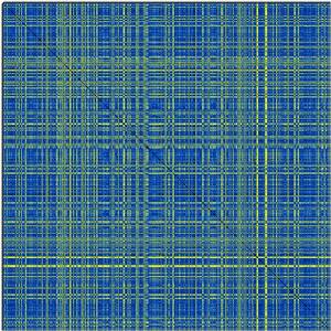
and view the resulting postscript file. If you wanted to use all heavy atoms of segid “P” and every 250th structure you would have said:
carma -v -cross -segid P -atmid HEAVY -step 250 my.dcd my.psf
Cluster analysis based on the distance (RMSD) matrix
Now, lets assume you have a crossDCD.matrix plot like the following and you wish to perform a cluster analysis of the RMSD matrix.

Performing cluster analysis based on a distance matrix has many possible solutions, and not a uniquely correct answer. Have a look at http://www.statmethods.net/advstats/cluster.html for things that can be done with the R package. One possible line of work (which assumes that you can decide at what RMSD cutoff you want to define clusters) is:
First, you make a dendrogram based on these RMSDs using the statistical package R and a hierarchical cluster analysis method, like hclust(). Before starting R, wc your matrix to find out its dimensions. Then:
#
#
# d -h
total 46M
-rw-r--r-- 1 glykos glykos  46M Mar 29 13:37 crossDCD.matrix
#
#
# wc -l crossDCD.matrix
2500 crossDCD.matrix
#
#
# R | tee LOG

R version 2.8.1 (2008-12-22)
Copyright (C) 2008 The R Foundation for Statistical Computing
ISBN 3-900051-07-0

R is free software and comes with ABSOLUTELY NO WARRANTY.
You are welcome to redistribute it under certain conditions.
Type 'license()' or 'licence()' for distribution details.

R is a collaborative project with many contributors.
Type 'contributors()' for more information and
'citation()' on how to cite R or R packages in publications.

Type 'demo()' for some demos, 'help()' for on-line help, or
'help.start()' for an HTML browser interface to help.
Type 'q()' to quit R.

> A <- matrix(scan("crossDCD.matrix", n = 2500*2500), 2500, 2500, byrow = TRUE)
Read 6250000 items
> hc <- hclust( as.dist(A), method="average")
> plclust(hc)
> postscript()
> plclust(hc)
> dev.off()
null device
> cutree( hc, h = 1.3)
   [1] 1 1 1 2 2 2 2 2 2 1 1 1 1 2 1 1 1 1 1 1 1 1 1 1 1 1 1 1 1 1 2 1 1 1 1 1 1
  [38] 1 1 1 1 1 1 1 2 2 2 1 1 1 2 2 1 1 1 1 1 1 1 1 1 1 1 1 1 1 2 1 1 2 2 1 1 1
  [75] 1 1 1 1 1 1 1 1 1 1 2 1 1 1 1 1 1 1 1 1 1 1 1 1 1 2 2 2 2 1 1 2 1 1 1 1 1
 [112] 1 2 1 1 2 2 1 1 1 2 2 2 2 1 2 1 1 2 1 1 1 1 1 1 1 1 1 1 2 2 2 1 1 1 1 2 2
 [149] 1 1 1 1 1 1 1 1 1 2 1 1 1 1 1 1 1 1 1 1 1 1 1 1 2 2 1 1 1 1 1 2 2 1 1 1 1
 [186] 1 2 1 1 1 2 2 1 1 1 1 1 1 1 1 1 1 1 1 1 1 1 1 1 1 1 1 1 1 1 1 1 1 1 1 1 1
 [223] 1 1 1 1 1 1 1 1 1 1 1 1 1 2 1 1 1 1 1 1 1 1 1 1 1 1 1 2 2 1 1 1 2 2 1 1 1
 [260] 1 2 2 2 1 1 1 1 1 1 1 1 1 1 1 2 1 1 1 1 1 1 1 1 1 1 1 2 2 1 1 1 1 1 1 2 2
 [297] 1 1 2 1 1 1 1 1 1 2 2 1 2 2 1 1 1 2 1 1 1 1 1 1 1 1 1 1 1 1 1 1 1 1 2 2 2
 [334] 1 1 1 1 1 2 2 2 2 2 1 1 1 1 1 1 1 2 1 1 1 1 1 2 1 1 1 1 1 1 2 2 1 1 1 1 1
                     <many lines with cluster assignments>
[2332] 1 1 1 1 1 1 1 1 1 1 2 2 1 2 1 1 2 1 1 1 1 1 1 1 1 1 1 1 1 1 2 2 1 2 2 1 1
[2369] 1 1 1 1 1 2 2 1 1 1 1 1 1 1 1 1 1 1 1 1 2 1 1 2 1 1 1 1 1 1 1 1 1 1 1 1 1
[2406] 1 2 2 3 2 1 1 1 1 1 2 2 1 1 1 1 1 1 1 1 2 1 1 1 1 1 1 1 1 1 1 1 1 1 1 2 2
[2443] 1 1 1 1 1 1 2 1 1 1 2 2 2 2 2 1 1 1 1 1 1 1 1 1 1 1 1 1 1 1 1 1 1 1 1 1 1
[2480] 1 2 2 1 1 1 1 2 2 2 1 1 2 2 1 2 2 1 1 1 1
> rect.hclust( hc, h = 1.3, border="red")
> clusters <- cutree( hc, h = 1.3)
> as.data.frame(clusters)
>q()
Save workspace image? [y/n/c]: n
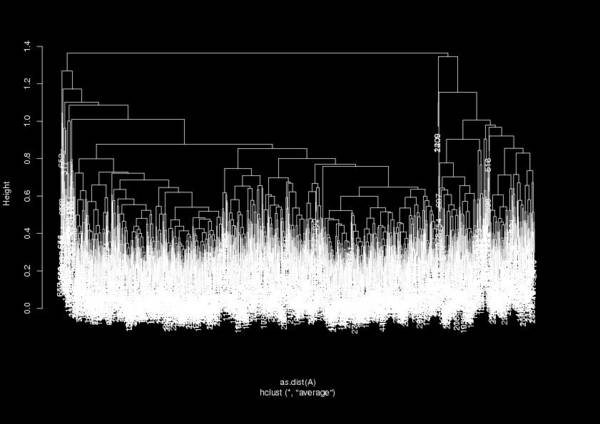
Which gives a dendrogram like:

From this dendrogram you can define a cutoff to find the number of clusters (the expression h = 1.3 in the example shown above). The variable as.data.frame(clusters) gives you something similar to the carma.clusters.dat file, where each frame is assigned to a cluster (per line). This way you can prepare a DCD file that corresponds to each cluster and continue your analysis from there…
OLD STUFF : Calculation of the RMSD matrix using crossDCD
Use the crossDCD script (from carma's distribution) to obtain a two-dimensional matrix with all frame-to-frame RMSDs of your trajectory (type 'crossDCD' from the shell for a usage summary). Adjust the step (for crossDCD) in such a way as to have manageable matrix sizes (max ~5000×5000). After the calculation finishes, the matrix will be contained in a file (in the current working directory) named crossDCD.matrix . You can plot the matrix with carma -col - < crossDCD.matrix . A typical session would look like this:
#
# d -h
total 2.0G
-r--r--r-- 1 glykos glykos 2.0G Mar 29 13:24 INYWLAH.dcd
-r--r--r-- 1 glykos glykos  30K Mar 29 13:24 INYWLAH.psf
#
# carma -v -w -fit -step 500 INYWLAH.dcd INYWLAH.psf

carma v.1.1____________________________________________________________________

7  CA   atoms are declared in the PSF file.
It appears that this DCD file contains unit cell information.
Number of coordinate sets is 1309323
Starting timestep         is 0
Timesteps between sets    is 1
Titles :
Created by DCD plugin
REMARKS Created 10 July, 2010 at 13:31
Number of atoms in sets   is 128
Fit DCD frames onto reference frame.
Now processing frame  1309500
End of DCD reached.
All done.
#
#
# d -h
total 2.0G
-r--r--r-- 1 glykos glykos 2.0G Mar 29 13:24 INYWLAH.dcd
-r--r--r-- 1 glykos glykos  30K Mar 29 13:24 INYWLAH.psf
-rw-r--r-- 1 glykos glykos 451K Mar 29 13:28 carma.fit-rms.dat
-rw-r----- 1 glykos glykos 420K Mar 29 13:28 carma.fitted.dcd
-rw-r--r-- 1 glykos glykos  811 Mar 29 13:28 carma.selected_atoms.psf
#
# mv carma.fitted.dcd CAs.dcd
# mv carma.selected_atoms.psf CAs.psf
# rm carma.fit-rms.dat
#
# d -h
total 2.0G
-rw-r----- 1 glykos glykos 420K Mar 29 13:28 CAs.dcd
-rw-r--r-- 1 glykos glykos  811 Mar 29 13:28 CAs.psf
-r--r--r-- 1 glykos glykos 2.0G Mar 29 13:24 INYWLAH.dcd
-r--r--r-- 1 glykos glykos  30K Mar 29 13:24 INYWLAH.psf
#
#
# crossDCD

Usage   : CrossDCD <PSF_file> <DCD_1> <DCD_2> [step] [flags]
Summary : Calculate a 2D matrix containing the rms  deviations
          (after  least  squares  fitting) between  the frames
          of two DCD files. If <step> is defined, then instead
          of using each and every frame of the  two DCDs, only
          consider every <step>th frame.  DCD_1 and  DCD_2 can
          well be the one and same file. The  matrix  will  be
          written to a  file ( crossDCD.matrix ).  To plot the
          results use 'carma - < crossDCD.matrix' and view the
          resulting postscript file.
          If you want to pass flags to the carma runs  (things
          line -segid or -atomid), you will have to define the
          <step> (even if it is 1)  and  then  define  carma's
          flags enclosed in double quotes (ie " ...flags...").

#
# crossDCD CAs.psf CAs.dcd CAs.dcd
DCD_1 and DCD_2 are identical. Will calculate intra-DCD rmsds.
DCD_1 contains 2619 frames
DCD_2 contains 2619 frames
..................................................
..................................................
             <many lines with dots>
..................................................
..................................................
...................
#
# d -h
total 2.1G
-rw-r----- 1 glykos glykos 420K Mar 29 13:28 CAs.dcd
-rw-r--r-- 1 glykos glykos  811 Mar 29 13:28 CAs.psf
-r--r--r-- 1 glykos glykos 2.0G Mar 29 13:24 INYWLAH.dcd
-r--r--r-- 1 glykos glykos  30K Mar 29 13:24 INYWLAH.psf
-rw-r--r-- 1 glykos glykos  46M Mar 29 13:37 crossDCD.matrix
#
# carma -col - < crossDCD.matrix
Will plot the gradient from 0.000000 to 5.753800 using colour postscript.
#
# wc -l crossDCD.matrix
2619 crossDCD.matrix
#
# d -h
total 2.1G
-rw-r----- 1 glykos glykos 420K Mar 29 13:28 CAs.dcd
-rw-r--r-- 1 glykos glykos  811 Mar 29 13:28 CAs.psf
-r--r--r-- 1 glykos glykos 2.0G Mar 29 13:24 INYWLAH.dcd
-r--r--r-- 1 glykos glykos  30K Mar 29 13:24 INYWLAH.psf
-rw-r--r-- 1 glykos glykos  41M Mar 29 13:37 carma.stdin.ps
-rw-r--r-- 1 glykos glykos  46M Mar 29 13:37 crossDCD.matrix
#
#
# gs carma.stdin.ps
GPL Ghostscript 8.62 (2008-02-29)
Copyright (C) 2008 Artifex Software, Inc.  All rights reserved.
This software comes with NO WARRANTY: see the file PUBLIC for details.
>>showpage, press <return> to continue<<
GS> quit
#
#


