Distance-matrix-based clustering of principal components (dPCA or cPCA)
The idea behind this method is to make an accurate dendrogram based on hierarchical clustering.
For starters
First of all, you need to have installed the R and some libraries. In the paradigm i will show you, i use the version 3.4.0 of R and the libraries (factoextra, FactoMineR, cluster and fpc).
Second, depending on the physical memory that is available on your computer, the number of the frames that you will be able to cluster will be restricted.
(The way to compute this is: physical memory needed= (number_of_frames * number_of_frames * 4) / (1024 * 1024 * 1024) Gb)
Now the real thing
*Place a copy of your carma_dPCA.dat or carma_PCA.dat in a clean directory.
*Considering that we have 4Gb RAM we would be able to cluster approximately ≈ 32,500 frames, but let's be realistic. So we will cluster 8,649 frames. Imagining that we have a file that contains 6,000,000 frames we will pick one every 693th frame.
# perl -ne 'print ((0 == $. % 693) ? $_ : "")' carma_dPCA.dat > selected.dat
*Run R in the same directory.
# R
R version 3.4.0 (2017-04-21) -- "You Stupid Darkness"
Copyright (C) 2017 The R Foundation for Statistical Computing
Platform: x86_64-pc-linux-gnu (64-bit)

R is free software and comes with ABSOLUTELY NO WARRANTY.
You are welcome to redistribute it under certain conditions.
Type 'license()' or 'licence()' for distribution details.

Natural language support but running in an English locale

R is a collaborative project with many contributors.
Type 'contributors()' for more information and
'citation()' on how to cite R or R packages in publications.

Type 'demo()' for some demos, 'help()' for on-line help, or
'help.start()' for an HTML browser interface to help.
Type 'q()' to quit R.

 >PCA <- read.table("selected.dat")
 >d <- dist(PCA, method="euclidean")
 >fit <- hclust(d, method="complete")
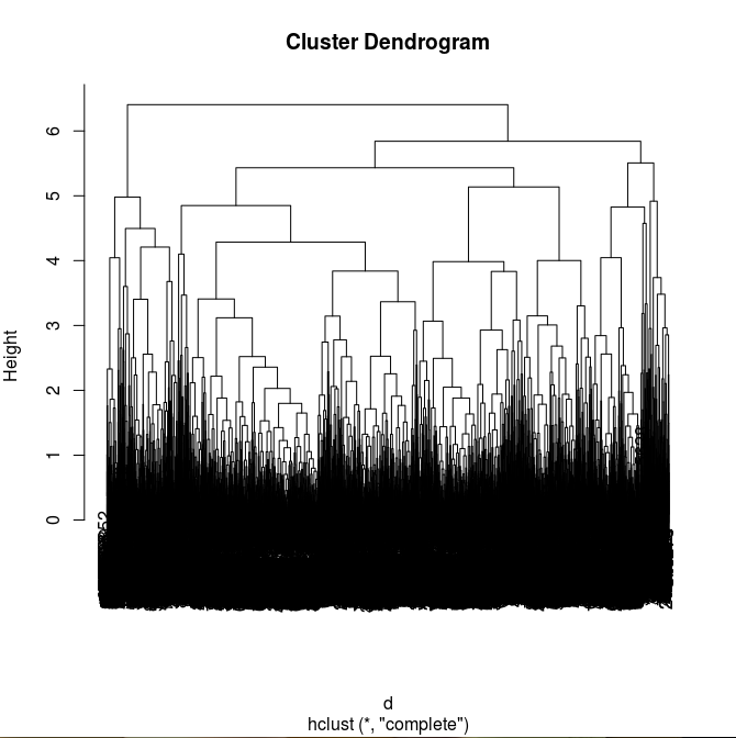
 >plot(fit)
 >q()
 >Save workspace image? [y/n/c]: n
Determining the optimal number of clusters
*We will use a considerable number of methods to ensure our options.
# R
R version 3.4.0 (2017-04-21) -- "You Stupid Darkness"
Copyright (C) 2017 The R Foundation for Statistical Computing
Platform: x86_64-pc-linux-gnu (64-bit)

R is free software and comes with ABSOLUTELY NO WARRANTY.
You are welcome to redistribute it under certain conditions.
Type 'license()' or 'licence()' for distribution details.

Natural language support but running in an English locale

R is a collaborative project with many contributors.
Type 'contributors()' for more information and
'citation()' on how to cite R or R packages in publications.

Type 'demo()' for some demos, 'help()' for on-line help, or
'help.start()' for an HTML browser interface to help.
Type 'q()' to quit R.

 >library(fpc)
 >library(factoextra)
 >library(cluster)
 >library("FactoMineR")
 >PCA <- read.table("selected.dat")
 >pamk.best <- pamk(PCA)
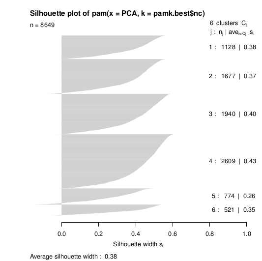
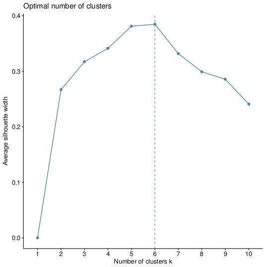
 >cat("number of clusters estimated by optimum average silhouette width: ", pamk.best$nc, "\n")
  number of clusters estimated by optimum average silhouette width: 6
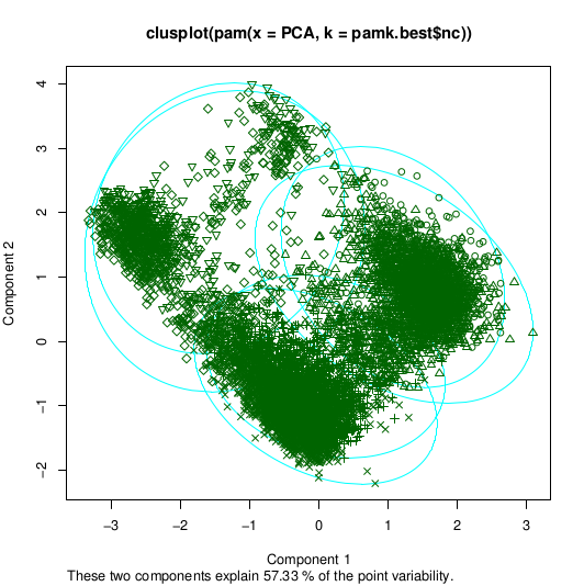
 >plot(pam(pca, pamk.best$nc))
 Hit <Return> to see next plot:<Return>
 Hit <Return> to see next plot:<Return>
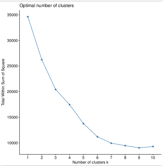
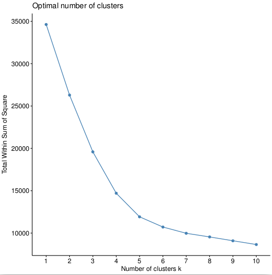
 >fviz_nbclust(pca, kmeans, method="wss")
 >fviz_nbclust(pca, pam, method="wss")
 >fviz_nbclust(pca, kmeans, method="silhouette")
 >fviz_nbclust(pca, pam, method="silhouette")
 >wss <- (nrow(pca)-1)*sum(apply(pca,2,var))
 >for (i in 2:15) wss[i] <- sum(kmeans(pca, centers=i)$withinss)
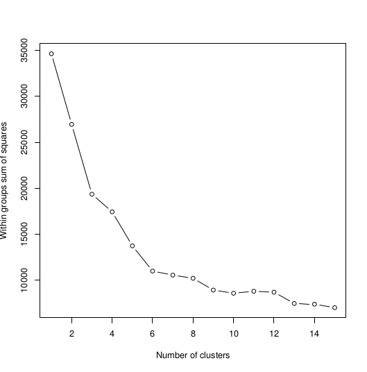
 >plot(1:15, wss, type="b", xlab="Number of Clusters", ylab="Within groups sum of squares")
 >q()
 >Save workspace image? [y/n/c]: n
Which will give us the plots, respectively:
So the optimal option is 6 clusters
Grand Finale
*We need to get the results in a document
# R
R version 3.4.0 (2017-04-21) -- "You Stupid Darkness"
Copyright (C) 2017 The R Foundation for Statistical Computing
Platform: x86_64-pc-linux-gnu (64-bit)

R is free software and comes with ABSOLUTELY NO WARRANTY.
You are welcome to redistribute it under certain conditions.
Type 'license()' or 'licence()' for distribution details.

Natural language support but running in an English locale

R is a collaborative project with many contributors.
Type 'contributors()' for more information and
'citation()' on how to cite R or R packages in publications.

Type 'demo()' for some demos, 'help()' for on-line help, or
'help.start()' for an HTML browser interface to help.
Type 'q()' to quit R.

 >PCA <- read.table("selected.dat")
 >d <- dist(PCA, method="euclidean")
 >fit <- hclust(d, method="complete")
 >groups <- cutree(fit, k=6)
 >tab <- data.frame(PCA, groups)
 >write.table(tab, file="PCA_Clusters.dat", sep=" ")
 >q()
 >Save workspace image? [y/n/c]: n
Which give us a file PCA_Clusters.dat, that has the frames and the clusters they belong at the end of each line.
By Alexander Chatzisavvas
Application when only a distance matrix is available
R version 3.2.3 (2015-12-10) -- "Wooden Christmas-Tree"
Copyright (C) 2015 The R Foundation for Statistical Computing
Platform: x86_64-pc-linux-gnu (64-bit)

R is free software and comes with ABSOLUTELY NO WARRANTY.
You are welcome to redistribute it under certain conditions.
Type 'license()' or 'licence()' for distribution details.

  Natural language support but running in an English locale

R is a collaborative project with many contributors.
Type 'contributors()' for more information and
'citation()' on how to cite R or R packages in publications.

Type 'demo()' for some demos, 'help()' for on-line help, or
'help.start()' for an HTML browser interface to help.
Type 'q()' to quit R.

> library(cluster)
> library(fpc)
> A <- matrix(scan("rmsd.mat", n = 2000*2000), 2000, 2000, byrow = TRUE)
Read 4000000 items
> data <- as.dist(A)
> pamk.best <- pamk(data, krange=2:10)
> plot(pam(data, pamk.best$nc))
> pam(data, pamk.best$nc)
Medoids:
       ID
[1,] 1180 1180
[2,]  518  518
[3,] 1786 1786
Clustering vector:
   [1] 1 1 1 1 1 1 1 1 1 1 1 1 1 1 1 1 1 1 1 1 1 1 1 1 1 1 1 1 1 2 2 2 1 1 1 1 1
  [38] 1 2 2 2 2 2 2 2 1 2 2 2 1 3 1 1 1 1 1 1 1 1 1 1 1 1 1 1 1 1 1 1 1 2 2 1 1

...............

[1888] 3 1 1 1 1 1 3 3 3 3 3 3 3 1 3 3 3 1 1 1 1 1 1 1 1 1 1 3 2 1 2 1 1 1 1 1 1
[1925] 1 1 1 1 1 1 1 1 1 1 1 1 1 1 1 1 1 1 1 1 1 1 1 1 1 1 1 1 1 1 1 1 1 1 1 1 1
[1962] 1 1 1 1 1 1 1 1 1 1 1 1 1 1 1 1 1 1 1 1 1 1 1 1 1 1 1 1 1 1 1 1 1 1 1 1 1
[1999] 1 1
Objective function:
   build     swap
2.397065 2.364252

Available components:
[1] "medoids"    "id.med"     "clustering" "objective"  "isolation"
[6] "clusinfo"   "silinfo"    "diss"       "call"
>


